Showing posts with label Boost.Geometry. Show all posts

Monday, May 8, 2023

Partition with Boost.Geometry

Partition with Boost.Geometry


Speeding up with divide and conquer

Boost.Geometry contains many algorithms in its official interface. Most of them follow the OGC interface specification, such as

  • distance
  • area
  • intersection
  • within

But there are also some other algorithms, which are mainly, or exclusively, used internally. One of them is partition and this blog post is about spatial partitioning. 

Suppose you have 1000 points and 1000 polygons, and you want to calculate how many points are within a polygon.

With Boost.Geometry that is easy: iterate over all points, for each of them iterate over all polygons, call the within algorithm, and if it returns true then increase the count. If polygons overlap, then one point might be in several polygons, but we ignore this for now (it’s trivial to fix).

It is easy but it can perform badly. Because it is a so-called “quadratic loop”. If there are, for example, just 10 elements, it is all fine. But if there are one million points and one million polygons, the within operation will be called one trillion times. Which is way too much.

The Boost.Geometry implementation, internally, often needs to compare such sets. For example, the intersection operation of two polygons starts with intersecting all segments of both polygons with each other. Walking over all segments of big polygons would be too slow.

To speed up this process, partition was implemented. It is similar to a kd-tree or to a quad-tree, but not identical. There is no data structure built, or kept. The space is recursively divided if necessary.

In more detail, it works as following:

  • the bounding box of the two sets are calculated
  • this box is divided into two halves, left and right
  • it takes the left half and tries to execute the operation there
But it is often, of course, still too much. In the figure below, the left half could be handled, maybe, but the right half contains for sure too many points.

It then continues:

  • the left box is divided into two halves, top and bottom
  • it takes the bottom half and tries to execute the operation there

This process goes on and on, dividing each box into two halves, alternating horizontally and vertically. Until there are a small number (16 by default) of points or polygons in the box. It then calls the specified operation, in this case within.

After the left half is completely handled, we get:

And after handling the right side, the very end of the process, we can see:

Some boxes are smaller than other boxes, because there are more points there (on purpose, the points are not distributed equally for this example), and/or more polygons.

The "operation" can be specified at compile time, like the compare algorithm in sorting. So in this case we can to calculate within for point-in-polygon, but in other cases we want to calculate intersections.

So, in summary, partition divides the space into halves, alternating left/right and top/bottom until there are just a few geometry objects, and then these geometries are fed into the specified operation.

Of course: if a box is divided into two halves, there can be polygons on the dividing line. They are in both the left and the right half. But this is recognized, and these polygons are handled separately, calling partition again but then for their bounding box.

If we compare calling the within operation with partition and with the trivial outer/inner loop implementation, we can see that it helps a lot ((all measurements on my Linux laptop, in release mode).
  • 2000 points and 2000 polygons:
    • partition takes about 5 ms 
    • loops version takes about 115 ms
  • 20000 points and 20000 polygons:
    • partition takes about 205 ms 
    • loops version takes about 11150 ms

The partition algorithm, for this example, is called as following. I'm showing the experimental version here, using lambda's (Boost.Geometry is written before lambda's existed - the "normal" function is still using a policy with an 'apply' method).

std::size_t count = 0;
boost::geometry::experimental::partition<box_type>(points, rings,
[](auto& box, auto const& point) { bg::expand(box, point); },
[](auto const& box, auto const& point) { return ! bg::disjoint(point, box); },
[](auto& box, auto const& item) { bg::expand(box, item.box); },
overlaps_ring,
[&count](auto const& p, auto const& ring_item)
{
if (bg::within(p, ring_item.ring))
{
count++;
}
return true;
});

The last lambda is the main operation and is only called for a points and polygons which are in the same partitioned box. bg is a shorthand for Boost.Geometry.
 
There are four other lambda's specified. That is because partition needs to calculate bounding boxes from its input (of which it is unaware, it can be anything, not even geometries but structures containing geometries, for example). Therefore, for the two input sets (points and rings) we need two additional lambda's (expanding a box with a point or ring, and returning true if a box intersects with a point or ring).

Wednesday, May 5, 2021

C++20 Concepts

C++20 Concepts


This week (2021) I'm at the C++Now conference. The conference is normally in Aspen, Colorado (I was there more than 10 years ago), but this year it's online, for obvious reasons.

Yesterday there were two excellent interesting talks from Jeff Garland about concepts in C++20, how it works, what you can do with it, how you can use them and how you can write them.

Some compilers (notably clang) don't yet support concepts, but you can already play with toy projects online using https://godbolt.org, where your code is compiled and run on the fly.

So here is my toy project, which I wrote during the talks (there were two consecutive talks):


#include <array>
#include <type_traits>
#include <iostream>

template <typename C> concept ValidCoordinateType = std::is_arithmetic_v<C>;
template <int D> concept ValidDimension = D >= 2 and D <= 3;
template <int D> concept HasZ = D >= 3;

template <typename C, int D>
requires(ValidDimension<D> and ValidCoordinateType<C>)
struct mypoint
{
  mypoint() = default;
 
  mypoint(C x, C y) 
    : coors{x, y} {}
 
  // Only available for 3D
  mypoint(C x, C y, C z) requires HasZ<D>
    : coors{x, y, z} {}
 
  auto x() const { return coors[0]; }
  auto y() const { return coors[1]; }

  // Avoids compilation for Dim < 3
  auto z() const requires HasZ<D> { return coors[2]; }
 
private :
   std::array<C, D> coors;
};

struct mytype {};

int main()
{
  mypoint<double, 2> two(1, 2);
  mypoint<float, 3> three(3, 4, 5);
  std::cout << "Hi " << two.x() << " " << two.y() << " " << three.z() << "\n";

  // These declarations will not compile
  //mypoint<mytype, 2> p1;
  //mypoint<double, 4> p2;
 
  // This line will not compile
  //std::cout << two.z(); // Fails because .z() is not available

  return 0;
}

So this code is using C++20 concepts. You can see it clearly at and around the keywords concept and requires. It is really cool, especially compared with what we had to do with C++03 (Boost.Geometry was written in C++03 and only a few releases ago went to C++14) to achieve this.

Some things could earlier be done with static_assert too (such as checking the number of dimensions), but now the compiler neatly warns that that is better written using a concept.

Other things needed SFINAE earlier (such as the enabling  / disabling the functions for the Z coordinate).

If the last declarations in main are uncommented, you get a neat compiler error report (for instance for p2):

<source>: In function 'int main()':
<source>:40:20: error: template constraint failure for 'template<class C, int D> requires (ValidDimension<D>) && (ValidCoordinateType<C>) struct mypoint'
40 | mypoint<double, 4> p2; // Fails because 4 coordinates are not allowed by the concept
| ^
<source>:40:20: note: constraints not satisfied
<source>:6:26: required for the satisfaction of 'ValidDimension<D>' [with D = 4]
<source>:6:56: note: the expression 'D <= 3 [with D = 4]' evaluated to 'false'
6 | template <int D> concept ValidDimension = D >= 2 and D <= 3;
| ~~^~~~

Wow, it's only a few lines! And so clear! In the past we got hundreds of hard to interpret error messages about templates...

And if you uncomment the line streaming z for a 2d coordinate, you get:

<source>: In function 'int main()':
<source>:43:22: error: no matching function for call to 'mypoint<double, 2>::z()'
43 | std::cout << two.z();
| ^
<source>:23:8: note: candidate: 'auto mypoint<C, D>::z() const requires HasZ<D> [with C = double; int D = 2]'
23 | auto z() const requires HasZ<D>
| ^
<source>:23:8: note: constraints not satisfied
<source>: In instantiation of 'auto mypoint<C, D>::z() const requires HasZ<D> [with C = double; int D = 2]':
<source>:43:22: required from here
<source>:7:26: required for the satisfaction of 'HasZ<D>' [with D = 2]
<source>:7:35: note: the expression 'D >= 3 [with D = 2]' evaluated to 'false'
7 | template <int D> concept HasZ = D >= 3;
| ~~^~~~

Wednesday, December 31, 2014

Vectorization with square point buffers

Vectorization with square point buffers


This year (2014) the buffer algorithm of Boost.Geometry was finally released in Boost 1.56

With buffer we mean a zone around a geometry. This is the GIS term, also used by OGC. In other environments it is often known as inflate / deflate, or shrink and expand, or Minkowski sum.

In GIS the buffer (with a positive distance) creates a larger version of e.g. a polygon. If a negative distance is specified, a smaller version is created.

As the documentation shows, various strategies can be used to:
  • control the buffer-distance (either symmetric or asymmetric)
  • control the joins (rounded or miter)
  • control the ends for linestrings (rounded or flat)
  • control the sides (straight)
  • control the zones around points (or degenerated linestrings) (circular or square)
Strategies are provided, but they can also be provided by the library user, e.g. to create some fancy effects.

This short blog gives an example of the strategies for zones around points, using the square version. This strategy has the nice property that can be used to convert grids or images to vectors (polygons).

strategy::buffer::point_square


See also the Wiki page. Pixels are converted to polygons. Suppose we add all centers of all filled pixels (e.g. the black pixels) into a multi point. We then buffer that multi-point with a distance of half the pixel size. And we use the strategy to create square buffers around each point. Then all adjacent gridcells will be connected. A polygon (or a multi-polygon) will be created, which is exactly what we wanted...

Suppose we have the following image (from this source) of a black cat.


Cat (pixels)

We create a multi-point of it, that is done manually:

MULTIPOINT(1 0,2 0,3 0,4 0,5 0,6 0,7 0,   0 1,1 1,2 1,3 1,4 1,5 1,7 1,8 1,  
0 2,1 2,2 2,3 2,4 2,5 2,8 2, 0 3,1 3,2 3,3 3,4 3,5 3,8 3,   0 4,1
4,2 4,3 4,4 4,5 4,8 4, 0 5,1 5,2 5,3 5,4 5,5 5,8 5,   1 6,2 6,3 6,4
6,7 6,8 6,   1 7,2 7,3 7,4 7,7 7, 1 8,2 8,3 8,4 8,7 8,   2 9,3
9,   6 9,7 9,   1 10,2 10,3 10,4 10,   1 11,2 11,3 11,4
11,   1 12,2 12,3 12,4 12,   1 13,4 13)

If we use the next code fragment:

    typedef boost::geometry::model::d2::point_xy<double> point;
    typedef boost::geometry::model::polygon<point> polygon;
    boost::geometry::strategy::buffer::distance_symmetric<double> distance_strategy(0.5);
    boost::geometry::strategy::buffer::join_round join_strategy;
    boost::geometry::strategy::buffer::end_round end_strategy;
    boost::geometry::strategy::buffer::point_square point_strategy;
    boost::geometry::strategy::buffer::side_straight side_strategy;
    boost::geometry::model::multi_polygon<polygon> result;
    boost::geometry::model::multi_point<point> mp;
    boost::geometry::read_wkt(cat, mp); // the cat std::string is somewhere defined
    boost::geometry::buffer(mp, result,
                distance_strategy, side_strategy,
                join_strategy, end_strategy, point_strategy);


The resulting polygon will look like this:

Cat (polygon)


Saturday, November 19, 2011

Linestring/polygon intersection


Linestring/polygon intersection


After a long while a blog again, a short one this time. I'm currently implementing intersections linestring/polygon for Boost.Geometry. Well, the basics (calculating intersection points) are already there for a long time, but for this combination the intersection points should be followed in another way and the correct pieces should be outputted.

When I do these things I normally check the results with both PostGIS and SQL Server. However, I'm encountering something weird in both of them.

The testcase

My testcase is looking like this:


SQL Server

In SQL Server the intersection is correctly done, but the linestring is reversed! I'm using this query:
with viewy as
(
   select
      geometry::STGeomFromText('POLYGON((1 1,1 3,3 3,3 1,1 1))', 0) as p,
      geometry::STGeomFromText('LINESTRING(2 2,1 2,1 3,2 3)', 0) as q
)
select
   p.STIntersection(q).STLength() as len,
   p.STIntersection(q).STAsText() as wkt
from viewy;

and this is my output:

3    LINESTRING (2 3, 1 3, 1 2, 2 2)

You see, the linestring is reversed! It is not only reversed with this linestring, but with all linestrings. Even if they are, for example, complete inside the polygon. If I reverse the polygon (from clockwise to counter clockwise), the output is still reversed. Mysterious...

PostGIS

Also a surprise in PostGIS.The query is looking there as following:

with viewy as
(
   select
      ST_GeomFromText('POLYGON((1 1,1 3,3 3,3 1,1 1))') as p,
      ST_GeomFromText('LINESTRING(2 2,1 2,1 3,2 3)') as q
)
select
   ST_Length(ST_Intersection(p, q)) as len,
   ST_AsText(ST_Intersection(p, q)) as wkt
from
viewy;
and this is here the result:

3;"MULTILINESTRING((1 2,1 3),(1 3,2 3),(2 2,1 2))"

I'm getting a multilinestring back! With respect to contents, it is OK. But it is surprising...

OGC

I did not look it up but I don't think this specific behaviour is specified. So yes, all implementations will be correct but...

Boost.Geometry

At the moment of writing, technically more difficult cases as this is one are not completely finished. But I can already tell that the linestring will not be reversed and that the output will consist of only one linestring...


Friday, June 24, 2011

Spherical Side Formula


Spherical Side Formula


This blog describes an algorithm and a formula to determine the side of one point relative to a segment (two other points), all three points located on a sphere.

The side informarmation is necessary for Boost.Geometry. It is used, among others, in the within algorithm, to check if a point is inside a polygon (point in polygon). With the spherical version of side, it can be checked if a point on a sphere (the earth) is inside a spherical polygon (e.g. a polygon measured in latitude, longitude).

It is also known as orientation (see also here and here)

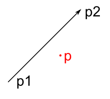
The Cartesian side is shown below. Point p is on the right side of segment p1-p2:
cs

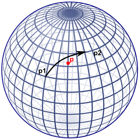
A visualization of ths spherical side is shown below, also here, point p is right of segment p1-p2.
ss

Note that if the cartesian side formula would be used on lat-long coordinates, this specific point would result on the left side.

Former approach

Boost.Geometry's former approach for spherical side used the useful aviation formulae of Williams, listed here. That did work but I was not completely satisfied about it:
  • it takes two * (3 cos, 3 sin, 1 atan) for the course, and then another 2 sin, and 1 asin, so in total 17 goniometric functions
  • it is non defined at the poles
  • I don't understand it fully, it seemed to me that there should be an easier way
An obvious alternative is translate to 3D cartesian coordinates and why not? After working this out a bit, it appeared that it indeed requires less goniometric functions. These goniometric functions are less performant and less precise, so if they can be avoided, the better. Also the new approach is also relatively easy, from mathematical perspective.

New approach

The new approach also uses sin and cos, but  less: for each of the points: 2 sin and 2 cos, in total 12 goniometric functions. Less then the former 17. More important, by design of Boost.Geometry, these might be precalculated such that for a spherical polygon it is not necessary to recalculate this again and again.

Besides that, the algorithm is easier to follow.

The algorithm

Let us calculate a plane through the two points of the segment, and the center of the sphere. This is the plane also containing the Great Circle. Let us then calculate at which side of the plane the point is located, either left of the plane, or right of the plane, or on the plane itself. The side with respect to the plane is also the side of the point with respect to the segment on the sphere.

To calculate a plane, all three points are transformed from spherical coordinates (longitude, latitude) to cartesian coordinates (x, y, z). Described a.o. here with clear images. We can use the unit sphere, it is not necessary to take the radius of the Earth (or another sphere or sphere-like object) into account. Amsterdam, for example, then lies somewhere here: (0.614161755 0.042946374 0.788010754).


Converting can conveniently be done using Boost.Geometry's transform algorithm (if p1 is stored in cs::spherical_equatorial):

        typedef model::point<coordinate_type, 3, cs::cartesian> point3d;
        point3d c1, c2, c3;
        transform(p1, c1);
        transform(p2, c2);
        transform(p, c3);
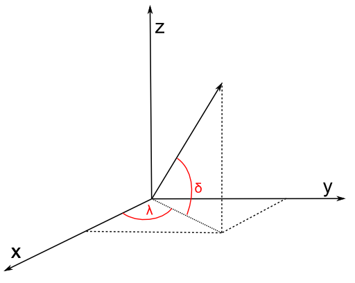
coordinate system

Then we define a plane through the center of the Earth (0,0,0) and the two points. We use the generalized plane equation for that (a x + b y + c z + d = 0), described e.g. here. This is done by taking the cross product of the two vectors (a vector is here: a mathematical vector). These two vectors are normally called v and w. Because we use (0,0,0) the points are the vectors, we don't have to subtract anything to create a vector. So v is equivalent to c1, w is equivalent to c2.

The cross product is the normal vector, called n, normal to the plane, so perpendicular to the great circle of the two points. So we can take the cross product:

vector_type const n = geometry::cross_product(v, w);

We now have our generalized plane equation. To make that explicit, we can use the conventional symbols a, b, c:

        coordinate_type const a = get<0>(n);
        coordinate_type const b = get<1>(n);
        coordinate_type const c = get<2>(n);

For the generalized plane equation, we should calculate d by subsituting one of the points going through the plane. Let us take (0,0,0)! By taking 0,0,0, all terms a x, b y, c z will be zero, so d is zero. Therefore we don't have to calculate d.

        double const d = 0;

The generalized plane equation has the property that, if you substitute another point, it is either on the plane (then the result = 0), or at one side of the plane (then the result is positive), or at another side of the plane (then the result is negative). Just like the Cartesian side, described above. And that is exactly what we need:

distance_measure = a * get<0>(c3) + b * get<1>(c3) + c * get<2>(c3) + d;

and we have the result:

int side
            = distance_measure > 0 ? 1 // left
            : distance_measure < 0 ? -1 // right
            : 0;

Spherical Side Formula

We used convenient vector calculation here, making it a mathematical exercise. Of course we could write them all out and get a lot of goniometric functions back.

One big note here: geographers (as I am) always refer to coordinates on a sphere by defining 0 at the equator. But mathematicians define 0 at the upper pole of a sphere. Watch out, it is different. This blog assumes the geographic convention, so assumes a spherical equatorial coordinate system.

Let's present it as mathematic formulae (thanks to mathcast):


The first formula converts to x,y,z. Be sure to enter all angles in radians. Also, be sure that λ is longitude (and comes first in Boost.Geometry) and δ is latitude (there are many conventions for this but I'm using them from here, and not from here and here and here). Latitude is 0 at the equator, 90 at the North Pole (again: mathematicians use 0 at the North Pole, 90 at the aquator; that is known as the spherical (polar) coordinate system, we now refer to the spherical equatorial coordinate system).

The second formula is the cross product and defines the terms of the generalized plane equation. The third formula calculates the distance measure (dm). Because (2) and (3) do not have repetitive clauses, they could be combined into (4) and then, if wished, again, with the conversion, into (5).

The sixth pseudo-formula then defines the result, it is an interpretation of the distance measure dm.

Ellipsoidal Earth

The Earth is not spherical but approximates an ellipsoid, it is flattened at the poles. But the described spherical side formula works well on Earth. Let me try to prove that (note: I'm a geographer, not a mathematician).

A location defined by (λδ) essentially means a vector, either on a sphere, or on an ellipsoid. These vectors always have the same direction, so the same on a sphere as on an ellipsoid. Their lengths differ (on an ellipsoid they are often shorter) but the length of a vector does not influence the plane it encompasses. Therefore the plane formed by two locations and the center of the Earth is exactly the same plane as it is using a perfect sphere.

So: two points (a segment), on a sphere or on an ellipsoid, define the same plane.

The same applies for the third point. It is also a vector, having a direction. That vector, either on a sphere or on an ellipsoid, is located at the same side of the plane.

Q.E.D.

Code

Because of the formulae above, I don't give (pseudo)code. It is quite easy. I created a small Excel sheet containing the formula is here. It contains this example (on this useful site): gcmap The formula is also in Boost.Geometry.

Summary

Using some high-school mathematics I presented an algorithm and a formula to calculate at which side a point is with resepect to a segment, on a sphere or on the Earth. Google did not find this for me. So I hope that it will be of some use for some people. At least, it is useful for Boost.Geometry

Wednesday, May 18, 2011

Debugger Visualizers


Debugger Visualizers


When debugging in Visual Studio, watching the contents of a variable can be of great help. But as soon as a variable is of a custom type, it might be inconvenient.

For example Boost.Geometry. You can examine the contents of a point or a polygon in the Debugger Watch Window. But the representation of a point type is cumbersome: "{...}". If you click that open, you will see m_values and a meaningless pointer. Still awkward. If you click that m_values open, you see it again, in the Values column the same pointer again. Still no coordinates. If you click that pointer open, yes, you finally see the values! But it takes three steps (clicks).

dv1

If you examine a polygon, you have to do these three steps for each point in each of its rings!

You will be tired of that soon, especially if you know it can be helped using the Visual Studio Debugger Visualizers. It seems this method is not documented by Microsoft, so it is a bit of hacking, but descriptions can be found on the web (references below).

This is the recipe how to do it:
  • go to the folder "c:\Program Files (x86)\Microsoft Visual Studio 10.0\Common7\Packages\Debugger" (usually there, path may change, this path is for VS 2010)
  • make a backup of the file autoexp.dat because we are going to change it
  • open autoexp.dat in an editor (it is (on Windows 7) convenient to edit in another path, because saving requires Administrator rights)
  • go to the bottom, just before [hresult]
  • enter the cryptic lines shown below this bullet list
  • save the file (if you did edit it in another path, copy it back, giving Administrator rights)
These are the lines to add:
boost::geometry::model::d2::point_xy<*,*>{
   preview ( #("(x=", $e.m_values[0], " ,y=", $e.m_values[1], ")") )
}
It is a bit abstruse. In preview ( #( ) ) you have to enter member variables of your class (which should be called $e for enigmatic reasons). You can mix them up with strings. All is comma separated. Note that the parentheses should be placed as displayed.

After this exercise, restart Visual Studio and debug again and... you will see a much better appearance of our point in the Watch window:

dv2
We don't have to click at all. Our point is just there, x- and y- coordinates specified. Oh yes, 4.56 is now 4.55999 but that is something different, it has to do with floating point precision. We ignore that in this blog.

Definition for Boost.Geometry

At this moment I have point_xy but also model::point defined. I could have more but this is already very useful. Linestrings or polygons automatically use these point presentations, and because std::vectors are visualized by Microsoft (in that same file autoexp.dat), it is all very clear in the Watch Window.

So the section I defined looks like this:

; BOOST.GEOMETRY

boost::geometry::model::point<*,2,*>{
   preview ( #("(", $e.m_values[0], " , ", $e.m_values[1], ")") )
}

boost::geometry::model::point<*,3,*>{
   preview ( #("(", $e.m_values[0], " , ", $e.m_values[1], " , ", $e.m_values[2], ")") )
}

boost::geometry::model::d2::point_xy<*,*>{
   preview ( #("(x=", $e.m_values[0], " ,y=", $e.m_values[1], ")") )
}
I have it running in Visual Studio C++ 2010 Express, and also in Visual Studio C++ 2005 Express. Debugging visualizers is a bit tricky, if you make an error you might get an exception window. But in version 2010 it is better than it was in version 2005.

References

There is more than this. More is explained on these pages: And in .NET (but this is actually another solution, implementing a custom visualizer in code):


Friday, May 6, 2011

SqlGeometry and Boxes


SqlGeometry and Boxes


I wanted to write a blog about partitioning (calling an algorithm using an on-the-fly quadtree or octree) and how it is implemented in Boost.Geometry, and how it could also be used / implemented for the SqlGeometry type. But somehow that blog will be too large and I blog here just about a box/rectangle in SqlGeometry. It is not too difficult, but I just googled and did not find other blogs saying the same things, so I hope it adds something.

STEnvelope


The OGC/ISO STEnvelope function, supported by spatial databases and many geometry libraries, returns the envelope of a geometry. An envelope is: a bounding box or bounding rectangle, also known as an axis aligned bounding box (aabb), a bbox, a minimum bounding rectangle (mbr) or an extent.

More in detail, STEnvelope returns a Geometry object describing a rectangle. OGC does not know the notion of a box. That is sometimes a bit inconvenient, but it is how it is. Boost.Geometry created a Box Concept, because Boost.Geometry is strongly typed, and envelopes returning polygons with always four or five points would confuse the non-OGC users of our library.

I blogged earlier about the spatial extent of a query in SQL Server, here.

A box is a simple geometry, with (in 2D) a minimum x and y and a maximum x and y. But how to get that from a geometry in a spatial database... I mean, the envelope returns a polygon containing five points (assuming it is closed), is the first point lower left? And is that guaranteed? The OGC specifications say: The minimum bounding box for this Geometry, returned as a Geometry. The polygon is defined by the corner points of the bounding box [(MINX, MINY), (MAXX, MINY), (MAXX, MAXY), (MINX, MAXY), (MINX, MINY)]. So yes, it should be guaranteed.

Let's look at it in more detail.

SQL Server


In SQL Server it indeed seems the case that the first point of the polygon returned by STEnvelope is the lower left point. Then, the third point must be the upper right point. Because, if you consider the polygon clockwise, it is the third point, and if it is counterclockwise, it is also the third point.

We use this query:

select geometry::STGeomFromText('POLYGON((0 0,2 5,4 1,0 0))',0).STEnvelope().STPointN(3).STAsText()

... to get the third point (which should be upper right), and it indeed gives me: POINT(4 5)

PostGIS


In PostGIS, the first point of the polygon returned by ST_Envelope is the lower left point as well. Great.

As you (maybe) know, SQLGeometry uses methods, PostGIS uses functions. So the corresponding nested function calls would be:

select ST_AsText(ST_PointN((ST_Envelope(ST_GeomFromText('POLYGON((0 0,2 5,4 1,0 0))',0))), 3))

But... no result, we get a null value back. Looking at the OGC specs, this is correct: NumPoints is defined for a LineString and not for a Polygon. SqlServer is somewhat more relaxed here (as is Boost.Geometry), returning the total number of points of a polygon (including interior rings, if any).

OK, behaviour is correct, so we try again, now inserting the ST_Boundary function (making a linestring of the boundary of a polygon). Our new function call is:

select ST_AsText(ST_PointN(ST_Boundary((ST_Envelope(ST_GeomFromText('POLYGON((0 0,2 5,4 1,0 0))',0)))), 3))

... and we have our upper right point. Using a 1 for the last value (the index of ST_PointN is one-based) would return the lower left point.

Boost.Geometry


Boost.Geometry, as said, returns a box (conforming a Box Concept) for the envelope (or assigns one). So this is more or less outside the discussion... Having a box you can get the minimum-corner coordinates (might be 2D, might be 3D, or more) and the maximum-corner coordinates.

SqlGeometry


I blogged about the useful SqlGeometry type here. The SqlGeometry type is polymorphic, it can be any OGC geometry. But, therefore, it cannot be a Rectangle (because, remember, a rectangle is not an OGC Geometry). So if it contains a Rectangle, it is a Polygon.

Using C#, it would be useful to get the coordinates from a Polygon returned by STEnvelope and that goes like this. Note that (in the light of defensive programming) we don't even assume that the first point is the lower left point. We add this code as a function (we could add it to a class GeometryExtensions, but for now we don't). It is called BoxToCoordinates, see the code below.

And, for symmetry, and because it is convenient, or often necessary (last reason most important ;-) ) we add a counterpart function as well, which creates a rectangle for you given four coordinate values. We call that one CoordinatesToBox, see code below.


The code


OK, this was some preparation for next blog, not too difficult, and now we can convert an STEnvelope result to coordinate values, and back. The full code is displayed below. Between BoxToCoordinates and CoordinatesToBox, there will be some more interesting calculations in the next blog. Stay tuned.

using System;
using Microsoft.SqlServer.Types;

namespace BlogSqlGeometryBox
{
    class Program
    {
        public static SqlGeometry FromWkt(string text, int srid)
        {
           return SqlGeometry.STGeomFromText(new System.Data.SqlTypes.SqlChars(text), srid);
        }

        public static SqlGeometry CoordinatesToBox(double x1, double y1, double x2, double y2, int srid)
        {
           SqlGeometryBuilder builder = new SqlGeometryBuilder();
           builder.SetSrid(srid);
           builder.BeginGeometry(OpenGisGeometryType.Polygon);
           builder.BeginFigure(x1, y1);
           builder.AddLine(x1, y2);
           builder.AddLine(x2, y2);
           builder.AddLine(x2, y1);
           builder.AddLine(x1, y1); // Yes, we close it neatly
           builder.EndFigure();
           builder.EndGeometry();
           return builder.ConstructedGeometry;
        }

        private static void MakeFirstSmaller<T>(ref T a, ref T b) where T : IComparable
        {
           if (a.CompareTo(b) > 0)
           {
               // Exchange the two values
               T t = a;
               a = b;
               b = t;
           }
        }

        public static void BoxToCoordinates(SqlGeometry box, out double x1, out double y1, out double x2, out double y2)
        {
           SqlGeometry lower_left = box.STPointN(1);
           SqlGeometry upper_right = box.STPointN(3);
           x1 = lower_left.STX.Value;
           y1 = lower_left.STY.Value;
           x2 = upper_right.STX.Value;
           y2 = upper_right.STY.Value;

           
// Defensive programming:
           MakeFirstSmaller(ref x1, ref x2);
           MakeFirstSmaller(ref y1, ref y2);
        }

        static void Main(string[] args)
        {
           SqlGeometry triangle = FromWkt("POLYGON((0 0,2 5,4 1,0 0))", 0);
           SqlGeometry box = triangle.STEnvelope();

           double x1, y1, x2, y2;
           BoxToCoordinates(box, out x1, out y1, out x2, out y2);

           // Do something with these coordinates. Let's create a larger box
           x1 -= 1;
           y1 -= 1;
           x2 += 1;
           y2 += 1;

           box = CoordinatesToBox(x1, y1, x2, y2, 0);

           System.Console.WriteLine(box.STAsText().ToSqlString().ToString());
        }
    }
}

Writing:

POLYGON ((-1 -1, -1 6, 5 6, 5 -1, -1 -1))

Saturday, February 19, 2011

Dissolving the Pentagram


Dissolving the Pentagram


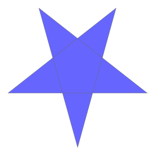
A week ago Denis asked the GGL-list if the internal segments of a self-intersecting polygon could be dropped. He attached this figure:
si

I answered that dissolve should do this. But it does not in this case. Dissolve can remove self-intersections, but under certain circumstances and even then it is not always perfect. So this is a reason to remove dissolve to the extensions folder - it should not yet be part of Boost.Geometry as it is released, hopefully in Boost 1.47

Pentagram

A pentagram is a five pointed star which can be drawn with a linestring of five segments. This is a Well-Known text presentation of a pentagram:

POLYGON((5 0,2.5 9,9.5 3.5,0.5 3.5,7.5 9,5 0))

As I often do, I compare the behaviour of algorithms on this WKT with SQL Server, PostGIS, and other packages (in this case Quantum GIS and SVG).

SVG

Boost.Geometry can create SVG images. This is really useful and I often use it in test programs. SVG's can then be depicted in FireFox. (In Google Chrome dropping the second SVG let it crash...).

SVG has thousands of properties, and one of them is the fill-rule. It can be set to winding and to non-zero. This delivers two different presentations:

winding non-zero
winding non-zero


SQL Server

In SQL Server the pentagram is drawn as such:

sql server
So it is using the winding rule.

The polygon is not valid, of course, it has five self-intersection points. SQL Server has a very good method to make polygons valid. It is obviously called MakeValid(). It is a SQL Server extension, not an OGC Method. I wrote "very good" and I mean that, we used it a lot in real-world problems and it has always worked very well.

With this specific pentagram MakeValid() creates a multi-polygon containing five triangles. So it directly uses the winding rule to create a multi-geometry. Sounds logical. If we calculate the area we get 17.7316840044235, the summed area of the five triangles. Calculating the area of a non-valid polygon is not possible in SQL Server. The statement is:

select geometry::STGeomFromText('POLYGON((5 0,2.5 9,9.5 3.5,0.5 3.5,7.5 9,5 0))',0)
.MakeValid().STArea()

PostGIS

PostGIS does not have a drawing engine. In PostGIS we can calculate the area of an invalid polygon and it gives us: 33.5. There is (AFAIK) not yet a function to make polygons valid, though it is announced. The good old trick is to use a buffer with buffer-distance 0, so we do this:

select ST_Area(ST_Buffer(ST_GeomFromText(
'POLYGON((5 0,2.5 9,9.5 3.5,0.5 3.5,7.5 9,5 0))',0),0))
and we get an area of 25.6158419936921. If we draw the zero-buffered result we get a filled polygon.

Boost.Geometry

Boost.Geometry can calculate the area of an invalid polygon and it also gives us: 33.5. The simple always-working Surveyor's formula just calculates this for us.

If we use the algorithm dissolve we indeed get a polygon with all internal corners dropped in this case. The area of the dissolved polygon is 25.6158412 and this is the right area. So the Surveyor's formula actually cannot be used with invalid polygons, SQL Server is right to prohibit this.

The SVG files displayed above are both created using Boost.Geometry so no picture here.

Quantum GIS

Quantum GIS has a great extension, QuickWKT, with which WKT geometries can be drawn. It uses the winding rule. It can calculate the area of the polygons (using the Info tool we can get it) and we get 33.5. Right, the Surveyor's formula.

qgis

What should happen

What should happen is not that simple. In these four programs, only SQL Server was consistent by prohibiting area calculation and creating a multi-geometry which looks like the image it depicts. All other programs and libraries were consistent, using the Surveyor's formula and creating a closed five-pointed polygon.

The reasoning of Boost.Geometry is that it takes direction into account. So if we draw arrows aside of all linestrings, we get:

arrowed

And here we see, in the triangle with the smaller arrows, that the direction is not consistent. That triangle should not be generated. Of this whole pentagram several polygons can be drawn with consistent directions, and the largest of them is the whole polygon. So the dissolve function is expected to generate a five-pointed star here. And it does.

There is also a pentagon in the center with consistent directions. Because it has the same orientation as the outer polygon, it should be discarded. And it is. If it would have been orientated counterclockwise, a hole should have been formed.

So there are reasons to say that this pentagram indeed should be converted into a solid five-pointed star. There is no winding rule or non-zero rule involved there, it is just derived by the directions of the segments created by the intersection.

But now the sample

Anyway, using the sample of Denis Pesotsky, Boost.Geometry's results were not that clever. It generates two polygons which are indeed as expected, with consistent directions. The outer polygon does not have a consistent direction and therefore should not be generated, correct. But there is one polygon with consistent direction missing, in the lower right. That one is discarded but should not have been...

denis

Because this, and because we have to think more about the behaviour, the dissolve algorithm has to be moved to the extensions folder. That means it will not be part of the initial release of Boost.Geometry, in the Release branch.

This is the WKT of the input polygon:

POLYGON((55 10, 141 237, 249 23, 21 171, 252 169, 24 89, 266 73, 55 10))

The white pieces are by the winding rule, and in SQL Server it is looking the same (no picture here). SQL Server's MakeValid() creates 9 polygons here.

PostGIS, using the buffer, creates one polygon, looking like this:
postgis

And that polygon is indeed the largest polygon which can be formed, following all arrows in clockwise direction. So this is the polygon that was expected by the dissolve algorithm...

Anyway, it is not the result that Denis asked for.

Useful usage

Dissolve can be very useful so I end this blog by just listing some of the testcases where it makes sense:

Inaccurate corners (extra intersection):
inaccurate corners


Messy corners:
dkn


Keyholed holes:
keyhole

Conclusions

Due to shortcomings in the dissolve algorithm and vagueness in behaviour in general we have to move the dissolve function to the extensions folder. It has to be thought over more thoroughly.


Sunday, February 13, 2011

Qt World Mapper with Boost.Geometry


Qt World Mapper with Boost.Geometry


Last year I created a simple world mapper using WxWidgets. For various reasons I decided to make the Qt equivalent as well.

Both Qt and WxWidgets are well-known cross-platform windows frameworks. Qt is used in Quantum GIS.

The World Mapper I created with WxWidgets did read world countries from a WKT (well-known text) file, and displayed them. Moving the mouse did highlight the country. For Qt it is similar (the highlighting is not yet been done).

The nice thing is that, by setting Boost.Geometry in this context, its force is shown:

Look below to lines marked with // Adapt. The QPointF and QPolygonF are just registered. From now on they act as normal Boost.Geometry geometries. So they can be used in area calculation, distance, transform, etc. We only use transform in this example.

So also look at lines commented with // This is the essention. Here a QPolygonF is declared, a ring (a normal Boost.Geometry part of a polygon, part of a multi-polygon) is transformed using the transformer to a QPolygonF. And the last one is of course displayed without any problem.

Delivering this application:

world


Complete C++ Code


#include <fstream> 

#include <QtGui>
#include <QWidget>
#include <QObject>
#include <QPainter>

#include <boost/foreach.hpp>

#include <boost/geometry/geometry.hpp>
#include <boost/geometry/geometries/register/point.hpp>
#include <boost/geometry/geometries/register/ring.hpp>

#include <boost/geometry/multi/multi.hpp>
#include <boost/geometry/extensions/algorithms/selected.hpp>
#include <boost/geometry/extensions/gis/io/wkt/wkt.hpp>

// Adapt a QPointF such that it can be handled by Boost.Geometry
BOOST_GEOMETRY_REGISTER_POINT_2D_GET_SET(QPointF, double, cs::cartesian, x, y, setX, setY)

// Adapt a QPolygonF as well.
// A QPolygonF has no holes (interiors) so it is similar to a Boost.Geometry ring
BOOST_GEOMETRY_REGISTER_RING(QPolygonF)

typedef boost::geometry::model::d2::point_xy<double> point_2d;
typedef boost::geometry::model::multi_polygon
    <
        boost::geometry::model::polygon<point_2d>
    > country_type;


class WorldMapper : public QWidget
{
public:
    WorldMapper(std::vector<country_type> const& countries, boost::geometry::model::box<point_2d> const& box)
        : m_countries(countries)
        , m_box(box)
    {
        setPalette(QPalette(QColor(200, 250, 250)));
        setAutoFillBackground(true);
    }

protected:
    void paintEvent(QPaintEvent*)
    {
        map_transformer_type transformer(m_box, this->width(), this->height());

        QPainter painter(this);
        painter.setBrush(Qt::green);

        BOOST_FOREACH(country_type const& country, m_countries)
        {
          typedef boost::range_value<country_type>::type polygon_type;
          BOOST_FOREACH(polygon_type const& polygon, country)
          {
          typedef boost::geometry::ring_type<polygon_type>::type ring_type;
         
ring_type const& ring = boost::geometry::exterior_ring(polygon);

          // This is the essention:
    
      // Directly transform from a multi_polygon (ring-type) to a QPolygonF
        
  QPolygonF qring;
          boost::geometry::transform(ring, qring, transformer);

    
      painter.drawPolygon(qring);
          }
       }
    }

private:
    typedef boost::geometry::strategy::transform::map_transformer
        <
          point_2d, QPointF,
          true, true
        > map_transformer_type;

     std::vector<country_type> const& m_countries;
     boost::geometry::model::box<point_2d> const& m_box;
};


class MapperWidget : public QWidget
{
public:
     MapperWidget(std::vector<country_type> const& countries, boost::geometry::model::box<point_2d> const& box, QWidget *parent = 0)
         : QWidget(parent)
     {
         WorldMapper* mapper = new WorldMapper(countries, box);

         QPushButton *quit = new QPushButton(tr("Quit"));
         quit->setFont(QFont("Times", 18, QFont::Bold));
         connect(quit, SIGNAL(clicked()), qApp, SLOT(quit()));

         QVBoxLayout *layout = new QVBoxLayout;
         layout->addWidget(mapper);
         layout->addWidget(quit);
         setLayout(layout);
     }

};


template <typename Geometry, typename Box>
inline void read_wkt(std::string const& filename, std::vector<Geometry>& geometries, Box& box)
{
    std::ifstream cpp_file(filename.c_str());
    if (cpp_file.is_open())
    {
        while (! cpp_file.eof() )
        {
          std::string line;
          std::getline(cpp_file, line);
          if (! line.empty())
          {
          Geometry geometry;
         
boost::geometry::read_wkt(line, geometry);
         
geometries.push_back(geometry);
         
boost::geometry::combine(box, boost::geometry::make_envelope<Box>(geometry));
          }
        }
    }
}

int main(int argc, char *argv[])
{
    std::vector<country_type> countries;
    boost::geometry::model::box<point_2d> box;
    boost::geometry::assign_inverse(box);
    read_wkt("../data/world.wkt", countries, box);

    QApplication app(argc, argv);
    MapperWidget widget(countries, box);
    widget.setWindowTitle("Boost.Geometry for Qt - Hello World!");
    widget.setGeometry(50, 50, 800, 500);
    widget.show();
    return app.exec();
}

Conclusions

With less than 160 lines of code, Qt and Boost.Geometry we showed how it can quite conveniently combine together.
The source is shown above and in SVN it can be found here.

Actually this application (and its WxWidgets counterpart) was for me the reason to start the shapefile research, which final conclusions still have to be drawn.

Sunday, January 30, 2011

Precision, the cause of spikes


Precision, the cause of spikes


This is a follow-up on my last blog. The spikey effects we have seen are perfectly explainable and understandable.

What we did was:
  1. cut a parcel in two pieces
    1. create a cutline and make a (nearly linear) cutting polygon of it (using buffer)
    2. subtract that cutline from the geometry, using STDifference
  2. keep one piece, using STGeometryN
  3. subtract that piece from the parcel, using STDifference
The result should be the discarded piece, but we got back two free spikes extra.

This short blog will explain this a little more and, as a side note, use just another SQL syntax for the same result.

Side note: with

The query from my previous blog can be rewritten much more elegantly using the with syntax:
with myquery as 
(
  select
    geometry::STGeomFromWKB(0x0103000000010000001A00000023DBF97EE316064146B6F3FDD32513415A643BDFD216064175931804E225134196438B6C52150641C976BE9F34261341F6285C8F06150641022B871641261341F853E3A5D3140641E17A14AE50261341B81E85EBFB120641A4703D8A142713414E6210584D120641AC1C5A64602713414E621058431106414E621058C9271341A01A2FDD1B11064121B07268D8271341F4FDD478571006411904560ECF271341448B6CE7DD0F06418195438BC1271341F6285C8F6A0F06413BDF4F0DA72713410E2DB29D360F06416F1283C091271341E5D022DB070F0641F6285C0F7227134160E5D022DA0E06416F1283404F271341448B6CE7D30E0641F853E3A52427134154E3A59BE60E06411904568E07271341643BDF4F0C0F0641D7A3703DFC2613414A0C022B100F064125068115FB26134191ED7C3F310F0641B6F3FDD4F42613414C378941F11006414A0C022BA0261341EC51B81ECC1206413BDF4F0D40261341022B87167514064125068115F1251341B4C876BE8C160641C74B37897F25134121B07268C6160641508D976E7525134123DBF97EE316064146B6F3FDD3251341,28992)
      as parcel,
    geometry::STGeomFromText('LINESTRING(180955 313700,180920 313740)', 28992).STBuffer(0.1)
      as cutline
)
select parcel.STDifference((select parcel.STDifference(cutline).STGeometryN(2) from myquery))
from myquery

The with clause is useful to avoid repeating pieces (as having the WKB twice), and is essential to do recursive queries. You define an inlined viewy thingy (here "myquery") and use it.

Both SQL Server and PostGreSQL support with queries. See also this link which explains with in depth.

Floating point precision

Floating points are really awful. Everyone knows that if you divide one by six (1/6) and multiply the result with six ((1/6) * 6) you should get one back. However, with floating points this is not always the case. You might get 0.9999999 back. If you try it, you might also get the correct 1.0 back. That is (according to this book) because intermediate results are stored in the floating point register of the CPU. So it is by chance that it is right. In reality it will be wrong.

See also this link and scroll to "Rounding errors can play havoc with math-intense programs". Adding ten 0.1 values will result into 0.99999999999999989. I repeated this and indeed this is the case with a double. With a float the result is 1.0000001192092896. With ttmath it is 1.0, but as soon as you do the same trick with eleven 1/11 additions, you might get 0.9999999999999999999999999999999 back, or 1.0, depending on which precision you specify. Using Boost.Rational you get always 1/1, guaranteed, because it calculates in another way. It uses fractions and keeps fractions all the time. That is great in this use case.

What then caused the spikes

Now that we realize again that floating points are awful, we investigate how imprecision causes the spikes. The damage happens in the first phase. The first STDifference is used to cut the parcel into two pieces.

See the picture below. The grid is the so-called floating point grid. The smallest difference in a 32 bits floating point value (1.175e-38) is depicted. Any point (with float) must be located on one of the gridpoints. (In reality the FP-grid is irregular, but the idea will be clear).

So in this case (in most cases), the intersection point happens to fall between the gridpoints... All the vertices of both input polygons are located on the gridpoints, of course. But the real intersection point does not. It is rounded to one of the four gridpoints. It is just by chance to which one it is rounded. So the rounded intersection point is located on a gridpoint.

a


Suppose it rounds to the point labeled "3". We then get a resulting polygon as partly depicted here:


b

The resulting polygon (in blue) is too small. There is a small piece of the original polygon which is not covered by this piece, at the north side, upperleft of point 3. Subtract this resulting polygon from the original and of course, you will get the spike. There is also a similar small piece at the east side but that will not create a visual effect in this use case.

There is no obvious solution. It is the same as adding ten times 0.1. You get too much or too little. These spikes are too little in the first phase, and after the second difference, the two resulting spikes are a bit too much. This explains that sometimes you get zero, sometimes you get one and sometimes you get two spikes. It is by chance. If the rounding would go to point "1" in the picture above, there would be no spike there.

The spikes are not the result of flawed logic, or wrong decisions somewhere. It is just the rounding.

Use ttmath if you want to minimize the chance on it. Or work around it, e.g. by buffering the result with a small value e.g. -0.000001. Boost.Geometry now has some algorithms to find spikes and remove them.

By the way, the nice trick on cutting a parcel into two pieces was introduced in our project by our partners from B3Partners. The project where this study is from extracted is the Portaal Natuur en Landschap

Conclusions

In this use case, spikes are the geometric visualization of floating point imprecision.