C++20 concepts and traits

Intro

I like writing libraries. In 2007 I refactored the heart of our library using types into a library using templates. This looked a bit like:

struct point { double x, y; };

and then some functions using these types (there was also a polygon, etc).

When I was satisfied with the results I submitted this as a preview to Boost. The general reaction was: interesting, but it is not concept based, and therefore not generic enough.

So I had to make the types concept based, but I didn't know what it was. And I found out that concepts were not yet supported by the language - so how could I use them... That became all clear, with help of reviewers and joiners. The library was refactored again into a concept based library, it was accepted and it is now known as Boost.Geometry.

Now (14 years later) the C++ language has support for concepts.

This blog is targeted to the approach Boost.Geometry uses. It uses traits to adapt normal structs or classes to concepts. Functions in the library use those concepts. 

The example in  this blog

We start again with a point, and a function calculating the distance:

struct point { double x, y; };

template <typename Point>
double distance_using_point(const Point& p1, const Point& p2)
{
  auto sqr = [](const double v) -> double { return v * v; };
  return std::sqrt(sqr(p1.x - p2.x) + sqr(p1.y - p2.y));
}

This function is template based but not generic. It only works for any point type having .x and .y member variables. But suppose it is not a member variable but a function .x(). Or you are using a std::array with two elements [0] and [1] (denoting x, y).

Traits as free functions

We will use traits for that. There are more ways to define and use traits. A first, concise way (not recommended! see below for a better version) is to just define free templated functions:

 

namespace point_traits

{

  template <typename P> double get_x(const P& p);

  template <typename P> double get_y(const P& p);

}

and these functions can then be specialized for the type:

 

namespace point_traits

{

  template<> inline double get_x<point>(const point& p) { return p.x; }

  template<> inline double get_y<point>(const point& p) { return p.y; }

}

And this works! Suppose you are to write a distance function, using these traits, it could look like this:

template <typename P1, typename P2>
double calculate_distance(const P1& p1, const P2& p2)

{

  auto sqr = [](const double x) -> double { return x * x; };

  return std::sqrt(sqr(point_traits::get_x<P1>(p1) - point_traits::get_x<P2>(p2))

                 + sqr(point_traits::get_y<P1>(p1) - point_traits::get_y<P2>(p2)));

}

If you use a std::array, then you can specialize it too:

namespace point_traits

{

  template<> inline double get_x<std::array<double, 2>>(const std::array<double, 2>& p) { return p[0]; }

  template<> inline double get_y<std::array<double, 2>>(const std::array<double, 2>& p) { return p[1]; }

}

And you can calculate the distance of two different types, for example:

  point mp{1, 1};

  std::array<double, 2> sa{2, 2};

  std::cout << calculate_distance(mp, sa) << std::endl;

It writes: 1.41421 as expected.

 

 

Evaluation of traits-as-free-functions 

These traits give the example already a kind of concept based look. And it works, but there are some problems:

• functions cannot be specialized partially - this can be inconvenient
• suppose we want floats too, and long doubles, and we want to have that coordinate type defined in a meta-function. Where to define it?
• suppose we forget a traits adaptation: there is not appearing any compiler error message! Because it knows the generic templated function, and will not complain. It gives a linker error.
• it is (therefore) not suitable for C++20 concepts 

The linker error, in case the specialization for point is forgotten or not right, will look like:

undefined reference to `double point_traits::get_x<point>(point const&) 

undefined reference to `double point_traits::get_y<point>(point const&) 

 

The linker just can't find these definitions. Compilation was fine. You can live with this, but there is a better alternative.

Concepts 

Now we will try to make a C++ 20 concept using these traits:

template <typename P> 

concept IsPoint = requires (P p) 

{ 

  point_traits::get_x<P>(p);

  point_traits::get_y<P>(p);

};

template <typename P1, typename P2>

requires IsPoint<P1> && IsPoint<P2>

double calculate_distance(const P1& p1, const P2& p2)

{

  // the same implementation

}

So we added, in bright magenta:

1. a new concept IsPoint. That concept tries to use the functions in namespace point_traits. If they are not there, the type P does not fulfill the concept.
2. a require clause decorating the distance function, stating that both point types should fulfill the IsPoint concept.

How cool is that!

However, even using this concept, there is the same linker error message. There is no neat compiler message about concepts, which we wished and maybe expected...

 

Traits as a struct 

To fix this, the traits can be modeled as structures. So we adapt the code, we introduce a structure (here replacing the namespace - but that is only for the sake of the sample - these struct traits are often placed in an own namespace). And the structure is short!

template <typename P> struct point_traits {};

So it is an empty structure. The magic happens in the specializations:

template<> struct point_traits<point> 

{

  static double get_x(const point& p) { return p.x; }

  static double get_y(const point& p) { return p.y; }

};

template<> struct point_traits<std::array<double, 2>> 

{

  static double get_x(const std::array<double, 2>& p) { return p[0]; }

  static double get_y(const std::array<double, 2>& p) { return p[1]; }

};

It looks nearly the same, just that now the struct is templatized with point or the std::array, instead of the free functions. And the free functions are now static member functions.

The concept is also similar, it's just the <P> part moving a bit left to the structure:

template <typename P> 

concept IsPoint = requires (P p) 

{ 

  point_traits<P>::get_x(p); 

  point_traits<P>::get_y(p); 

};

And so does the final generic concept-based distance function:

template <typename P1, typename P2>

requires IsPoint<P1> && IsPoint<P2>

double calculate_distance(const P1& p1, const P2& p2)

{

  auto sqr = [](const double x) -> double { return x * x; };

  return std::sqrt(sqr(point_traits<P1>::get_x(p1) - point_traits<P2>::get_x(p2)) 

                 + sqr(point_traits<P1>::get_y(p1) - point_traits<P2>::get_y(p2)));

}

And if we now forget a specialization? We get a neat error message. In clang (13) it reads:

prog.cc:62:16: error: no matching function for call to 'calculate_distance'
  std::cout << calculate_distance(mp, sa) << std::endl;
               ^~~~~~~~~~~~~~~~~~
prog.cc:45:8: note: candidate template ignored: constraints not satisfied [with P1 = point, P2 = std::array<double, 2>]
double calculate_distance(const P1& p1, const P2& p2)
       ^
prog.cc:43:10: note: because 'point' does not satisfy 'IsPoint'
requires IsPoint<P1> && IsPoint<P2>
         ^
prog.cc:35:20: note: because 'point_traits<P>::get_x(p)' would be invalid: no member named 'get_x' in 'point_traits<point>'
  point_traits<P>::get_x(p); 
                   ^
1 error generated. 

 

You can use C++20 and concepts, for example, in Wandbox.

Samples from libraries

Boost.Geometry uses this approach, also generalized for coordinate type and dimension. Here is the adaptation of the get function for std::array (in namespace boost::geometry::traits). It's partially specialized.

 

template <typename CoordinateType, std::size_t DimensionCount, std::size_t Dimension>

struct access<std::array<CoordinateType, DimensionCount>, Dimension>

{

    static inline CoordinateType get(std::array<CoordinateType, DimensionCount> const& a)

    {

        return a[Dimension];

    }

};

MapBox uses a similar approach, here is the adaptation for our point (in namespace mapbox::util):

template <> struct nth<0, point> 

{

  inline static auto get(const point &t) { return t.x; }

};

template <> struct nth<1, point> 

{

  inline static auto get(const point &t) { return t.y; }

};

Summary

The blog above shows, shortly, how to define traits, preferably as structs, and how to define a concept and use this concept in a free function distance.

SQLite, Ado.Net, SpatiaLite

SQLite is a small but great database. SpatiaLite is its spatial extension. ADO.NET is the method to access databases in .NET.

This blog shows how to combine them, because I did found all information on the web but not a complete and up-to-date story.

SQLite and Ado.Net

An introduction (up and running in 3 minutes) is here. It is good but not up-to-date. In the meantime the ADO.NET driver is transferred from sourceforge/phxsoftware to sqlite.org, which is of course a good sign.

There is only one piece of software which you really need and that is the ADO.NET driver. Furthermore there are some optional (but very useful tools) which I describe below.

ADO.NET driver

The current ADO.NET driver page is here, and more specificly you can download the drivers from this page. Download for example the sqlite-netFx40-setup-bundle-x86-2010-1.0.77.0.exe (10.25 MiB)  (at least I did) and install it. The installation folder will contain the driver, and also a manual and a sample database (northwindEF.db).

Setting up the project

Create a new project (or use an existing) in C# Express or Visual Studio (I'm using 2010). I created a Console Project.

Most important is of course to add a reference. Typically you need  the System.Data.SQLite.dll from the installation folder (typically "c:\Program Files (x86)\System.Data.SQLite\2010\bin" ). You can either reference it from there or copy it to your project folder and reference it.

Writing the code.

See also the original 3 minutes introduction for some code. Here a different sample is presented. I like complete code and I also include some extra optional pieces which I needed (creating a new database from scratch, and turning on foreign keys).

So a complete program looks like:

// Copyright (c) 2011 Barend Gehrels 
using System; 
using System.Data.Common; 
using System.Data.SQLite; 

namespace SQLiteAndAdoDotNet 
{ 
    class Program 
    { 
        const string mydb = @"c:\temp\mydatabase.db"; 

        static void Main(string[] args) 
        { 
            bool isNew = false;

            if (!System.IO.File.Exists(mydb)) 
            { 
                // Create a new SQLite database if it does not exist
                SQLiteConnection.CreateFile(mydb); 
                isNew = true; 
            } 

            using (SQLiteConnection connection = new SQLiteConnection(@"Data Source=" + mydb)) 
            { 
                connection.Open(); 

                // Recommended action for any SQLite database
                ExecuteStatement("PRAGMA foreign_keys = ON", connection); 

                if (isNew) 
                { 
                    // Create a table for a new database 
                    ExecuteStatement(@" 
                        create table mytable 
                            ( 
                                id integer primary key autoincrement, 
                                myfield text, 
                                mydate integer -- dates can be stored as either text, real or integer 
                            ) 
                        ", connection); 
                } 

                // Insert something 
                ExecuteStatement("insert into mytable(myfield,mydate) values('my row',date('now'))", 
                    connection); 

                // Retrieve something 
                using (SQLiteCommand command = new SQLiteCommand("select *,datetime(mydate) as dt_ok from mytable", 
                            connection)) 
                { 
                    using (DbDataReader reader = command.ExecuteReader())
                    { 
                        while (reader.Read()) 
                        { 
                            System.Console.WriteLine(String.Format( 
                                "Row id={0} field={1} date={2}, dt={3}", 
                                reader["id"], reader["myfield"], 
                                reader["mydate"], reader["dt_ok"])); 
                        } 
                    } 
                } 
            } 
            System.Console.WriteLine("Done"); 
        } 

        private static void ExecuteStatement(string statement, SQLiteConnection connection)
        { 
            using (SQLiteCommand command = new SQLiteCommand(statement, connection))
            { 
                command.ExecuteNonQuery(); 
            } 
        } 
    } 
} 

I factored out one method to avoid repetitions. In another blog I'll show you a different approach.

The foreign key pragma is of course not necessary in this short sample. But in a "real" database, with a datamodel and foreign keys, you will need it. Otherwise cascaded deletes will fail unexpectedly!

One caveat

Beware for datetime fields, stored as real or integer! SQLite stores date types in any field, which is reasonable. But if you select such a date(time) field in the normal way you will get only the year back! So alas you have to cast it with the SQLite datetime function (described here). Dates stored as text do not have this caveat.

Useful tools

I like the SQLite Studio which can be downloaded freely from here. You can hardly without such a tool and this one is really cool. If you are coming from SQL Server you might also like a converter, and this one is good, free, and with source.

Using SpatialLite

Using SpatialLite is pretty much the same, from ADO.NET perspective. But of course you have to download some extra libraries. The SpatialLite library of course, but you also need at least two extra libraries. So here we go (see also StackOverflow):

• download the SpatiaLite DLL from this page (libspatialite-win-x86-2.3.1.zip)
• download proj-win as well from the same page (proj-win-x86-4.6.1.zip)
• download iconv as well from the same page (libiconv-win-x86-1.9.2.zip)
• download geos as well from the same page (geos-win-x86-3.1.1.zip) (I added geos later, after the comment of rmales, for me it was not necessary because it was found in my path, via PostGIS.)

But them all into your binary folder (Debug and Release). For our test project we also need a spatial database. You can create one from a shapefile (using the spatialite-gui from the same page) or download a test database from SpatialLite, here. I downloaded and extracted world.7z because I like to see world countries (see my other blogs).

Then, before you have to use it, you have to load the extension. That is pretty easy with an SQL statement, select load_extension('libspatialite-1.dll'). If it finds this DLL and the other two, it will run fine (and otherwise it will mention which is missing). Alas I could not get it working in sqlitestudio.

Then below is the program I used, and it runs fine. It is quite similar to the one above but I prefer to list it completely again. In next blog(s) we will do other interesting and maybe surprising things with it.

// Copyright (c) 2011 Barend Gehrels 
using System; 
using System.Data.Common; 
using System.Data.SQLite; 

namespace SQLiteAndAdoDotNet 
{ 
    class Program 
    { 
        const string mydb = @"c:\bdata\blogs\data\world.sqlite"; 

        static void Main(string[] args) 
        { 
            using (SQLiteConnection connection = new SQLiteConnection(@"Data Source=" + mydb)) 
            { 
                connection.Open(); 

                // Recommended action for any SQLite database
                ExecuteStatement("PRAGMA foreign_keys = ON", connection); 

                // Required action for any SpatiaLite database
                ExecuteStatement("select load_extension('libspatialite-1.dll')", connection); 

                // Retrieve some cities in Europe 
                using (SQLiteCommand command = new SQLiteCommand(
                        @" 
                            select wup_aggl,AsText(Geometry) as wkt,
                                X(Geometry) as x,Y(Geometry) as y
                            from Cities 
                            where MBRContains(BuildMBR(-2,40,10,80),Geometry) = 1 
                        ", connection)) 
                { 
                    using (DbDataReader reader = command.ExecuteReader())
                    { 
                        while (reader.Read()) 
                        { 
                            System.Console.WriteLine(String.Format( 
                                "City: {0} location: {1}, {2} wkt: {3}", 
                                reader["wup_aggl"], reader["x"], reader["y"], reader["wkt"])); 
                        } 
                    } 
                } 
            } 
            System.Console.WriteLine("Done"); 
        } 

        private static void ExecuteStatement(string statement, SQLiteConnection connection)
        { 
            using (SQLiteCommand command = new SQLiteCommand(statement, connection))
            { 
                command.ExecuteNonQuery(); 
            } 
        } 

    } 
} 

Useful tools

Of course you can use Quantum GIS to perfectly visualize your SpatiaLite database. The SpatiaLite page also contains many useful links.

Summary

Above two complete programs to use SQLite and/or SpatiaLite in your .NET application. This is the C# version, VB.NET will work either.

Linestring/polygon intersection

After a long while a blog again, a short one this time. I'm currently implementing intersections linestring/polygon for Boost.Geometry. Well, the basics (calculating intersection points) are already there for a long time, but for this combination the intersection points should be followed in another way and the correct pieces should be outputted.

When I do these things I normally check the results with both PostGIS and SQL Server. However, I'm encountering something weird in both of them.

The testcase

My testcase is looking like this:

SQL Server

In SQL Server the intersection is correctly done, but the linestring is reversed! I'm using this query:

with viewy as
(
   select
      geometry::STGeomFromText('POLYGON((1 1,1 3,3 3,3 1,1 1))', 0) as p,
      geometry::STGeomFromText('LINESTRING(2 2,1 2,1 3,2 3)', 0) as q
)
select
   p.STIntersection(q).STLength() as len,
   p.STIntersection(q).STAsText() as wkt
from viewy;

and this is my output:

3    LINESTRING (2 3, 1 3, 1 2, 2 2)

You see, the linestring is reversed! It is not only reversed with this linestring, but with all linestrings. Even if they are, for example, complete inside the polygon. If I reverse the polygon (from clockwise to counter clockwise), the output is still reversed. Mysterious...

PostGIS

Also a surprise in PostGIS.The query is looking there as following:

with viewy as
(
   select
      ST_GeomFromText('POLYGON((1 1,1 3,3 3,3 1,1 1))') as p,
      ST_GeomFromText('LINESTRING(2 2,1 2,1 3,2 3)') as q
)
select 
   ST_Length(ST_Intersection(p, q)) as len,
   ST_AsText(ST_Intersection(p, q)) as wkt 
from viewy;

and this is here the result:

3;"MULTILINESTRING((1 2,1 3),(1 3,2 3),(2 2,1 2))"

I'm getting a multilinestring back! With respect to contents, it is OK. But it is surprising...

OGC

I did not look it up but I don't think this specific behaviour is specified. So yes, all implementations will be correct but...

Boost.Geometry

At the moment of writing, technically more difficult cases as this is one are not completely finished. But I can already tell that the linestring will not be reversed and that the output will consist of only one linestring...

Spherical Side Formula

This blog describes an algorithm and a formula to determine the side of one point relative to a segment (two other points), all three points located on a sphere.

The side informarmation is necessary for Boost.Geometry. It is used, among others, in the within algorithm, to check if a point is inside a polygon (point in polygon). With the spherical version of side, it can be checked if a point on a sphere (the earth) is inside a spherical polygon (e.g. a polygon measured in latitude, longitude).

It is also known as orientation (see also here and here)

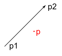
The Cartesian side is shown below. Point p is on the right side of segment p1-p2:


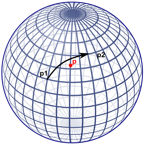
A visualization of ths spherical side is shown below, also here, point p is right of segment p1-p2.


Note that if the cartesian side formula would be used on lat-long coordinates, this specific point would result on the left side.

Former approach

Boost.Geometry's former approach for spherical side used the useful aviation formulae of Williams, listed here. That did work but I was not completely satisfied about it:

• it takes two * (3 cos, 3 sin, 1 atan) for the course, and then another 2 sin, and 1 asin, so in total 17 goniometric functions
• it is non defined at the poles
• I don't understand it fully, it seemed to me that there should be an easier way

An obvious alternative is translate to 3D cartesian coordinates and why not? After working this out a bit, it appeared that it indeed requires less goniometric functions. These goniometric functions are less performant and less precise, so if they can be avoided, the better. Also the new approach is also relatively easy, from mathematical perspective.

New approach

The new approach also uses sin and cos, but  less: for each of the points: 2 sin and 2 cos, in total 12 goniometric functions. Less then the former 17. More important, by design of Boost.Geometry, these might be precalculated such that for a spherical polygon it is not necessary to recalculate this again and again.

Besides that, the algorithm is easier to follow.

The algorithm

Let us calculate a plane through the two points of the segment, and the center of the sphere. This is the plane also containing the Great Circle. Let us then calculate at which side of the plane the point is located, either left of the plane, or right of the plane, or on the plane itself. The side with respect to the plane is also the side of the point with respect to the segment on the sphere.

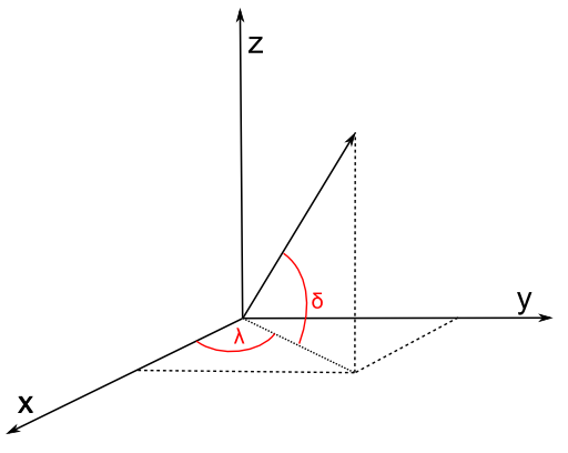
To calculate a plane, all three points are transformed from spherical coordinates (longitude, latitude) to cartesian coordinates (x, y, z). Described a.o. here with clear images. We can use the unit sphere, it is not necessary to take the radius of the Earth (or another sphere or sphere-like object) into account. Amsterdam, for example, then lies somewhere here: (0.614161755 0.042946374 0.788010754).


Converting can conveniently be done using Boost.Geometry's transform algorithm (if p1 is stored in cs::spherical_equatorial):

        typedef model::point<coordinate_type, 3, cs::cartesian> point3d;
        point3d c1, c2, c3;
        transform(p1, c1);
        transform(p2, c2);
        transform(p, c3);



Then we define a plane through the center of the Earth (0,0,0) and the two points. We use the generalized plane equation for that (a x + b y + c z + d = 0), described e.g. here. This is done by taking the cross product of the two vectors (a vector is here: a mathematical vector). These two vectors are normally called v and w. Because we use (0,0,0) the points are the vectors, we don't have to subtract anything to create a vector. So v is equivalent to c1, w is equivalent to c2.

The cross product is the normal vector, called n, normal to the plane, so perpendicular to the great circle of the two points. So we can take the cross product:

vector_type const n = geometry::cross_product(v, w);

We now have our generalized plane equation. To make that explicit, we can use the conventional symbols a, b, c:

        coordinate_type const a = get<0>(n);
        coordinate_type const b = get<1>(n);
        coordinate_type const c = get<2>(n);

For the generalized plane equation, we should calculate d by subsituting one of the points going through the plane. Let us take (0,0,0)! By taking 0,0,0, all terms a x, b y, c z will be zero, so d is zero. Therefore we don't have to calculate d.

        double const d = 0;

The generalized plane equation has the property that, if you substitute another point, it is either on the plane (then the result = 0), or at one side of the plane (then the result is positive), or at another side of the plane (then the result is negative). Just like the Cartesian side, described above. And that is exactly what we need:

distance_measure = a * get<0>(c3) + b * get<1>(c3) + c * get<2>(c3) + d;

and we have the result:

int side
            = distance_measure > 0 ? 1 // left
            : distance_measure < 0 ? -1 // right
            : 0;

Spherical Side Formula

We used convenient vector calculation here, making it a mathematical exercise. Of course we could write them all out and get a lot of goniometric functions back.

One big note here: geographers (as I am) always refer to coordinates on a sphere by defining 0 at the equator. But mathematicians define 0 at the upper pole of a sphere. Watch out, it is different. This blog assumes the geographic convention, so assumes a spherical equatorial coordinate system.

Let's present it as mathematic formulae (thanks to mathcast):



The first formula converts to x,y,z. Be sure to enter all angles in radians. Also, be sure that λ is longitude (and comes first in Boost.Geometry) and δ is latitude (there are many conventions for this but I'm using them from here, and not from here and here and here). Latitude is 0 at the equator, 90 at the North Pole (again: mathematicians use 0 at the North Pole, 90 at the aquator; that is known as the spherical (polar) coordinate system, we now refer to the spherical equatorial coordinate system).

The second formula is the cross product and defines the terms of the generalized plane equation. The third formula calculates the distance measure (dm). Because (2) and (3) do not have repetitive clauses, they could be combined into (4) and then, if wished, again, with the conversion, into (5).

The sixth pseudo-formula then defines the result, it is an interpretation of the distance measure dm.

Ellipsoidal Earth

The Earth is not spherical but approximates an ellipsoid, it is flattened at the poles. But the described spherical side formula works well on Earth. Let me try to prove that (note: I'm a geographer, not a mathematician).

A location defined by (λ, δ) essentially means a vector, either on a sphere, or on an ellipsoid. These vectors always have the same direction, so the same on a sphere as on an ellipsoid. Their lengths differ (on an ellipsoid they are often shorter) but the length of a vector does not influence the plane it encompasses. Therefore the plane formed by two locations and the center of the Earth is exactly the same plane as it is using a perfect sphere.

So: two points (a segment), on a sphere or on an ellipsoid, define the same plane.

The same applies for the third point. It is also a vector, having a direction. That vector, either on a sphere or on an ellipsoid, is located at the same side of the plane.

Q.E.D.

Code

Because of the formulae above, I don't give (pseudo)code. It is quite easy. I created a small Excel sheet containing the formula is here. It contains this example (on this useful site): gcmap The formula is also in Boost.Geometry.

Summary

Using some high-school mathematics I presented an algorithm and a formula to calculate at which side a point is with resepect to a segment, on a sphere or on the Earth. Google did not find this for me. So I hope that it will be of some use for some people. At least, it is useful for Boost.Geometry

Intersections (1)

The boolean operations are probably the most interesting parts of the Boost.Geometry library.

Boolean operations are, based on two polygons:

• intersection, returning polygons containing areas present in both input polygons
• union, returning polygons containing all areas present in either one of the input polygons
• difference, returning polygons containing areas present in one of the input polygons, but not in the other
• symmetric difference, returning polygons containing areas present in one of either input polygons, but not in both

In other words, boolean operations are spatial implementations of mathematical set theoretic operations. Based on two polygons A and B:

• intersection: A and B, also written as A ∩ B
• union: A or B, also written as A ∪ B
• difference: A and not B, also written as A \ B
• symmetric difference: A xor B, also written as A ∆ B

The difference operation (also known as relative complement) is the only operation of these which is not commutative, A \ B results in another geometry than B \ A. 

The basics

This blog will not explain the whole algorithm, that would be way too long. Other of my future blogs or a future article will explain more details. The algorithm used in Boost.Geometry is an adapted version of the Weiler-Atherton algorithm. The basics are quite simple, and explained here, and also in adapted versions as from Greiner-Hormann. Note that I have adapted the algorithm myself, such that intersection points are not inserted in the originals but stored separately. Which is essential because we don't want to change the input polygons, and we neither want to copy the input polygons. I have made more adaptations, such that all situations including self-tangencies (in some articles called degenerations) and robustness are handled.

So only the very basics in this blog. There are two input polygons, A and B (here: green and blue), both oriented clockwise. The arrows indicate orientation at the starting points. Intersection points (orange) are calculated. During the calculation of the intersection points, traversal information is gathered: for an intersection (usually: go to the right), would it continue following the green or the blue outline... For example, at point 0, above, it is figured out that for an intersection the green line should be followed, and for a union the blue line. Both until the next intersection point is encountered. That requires sorting which is used heavily within the algorithm.

Turning right for intersections or left for unions is also visualized below, from an older part of the GGL-doc:



How traversal information is figured out, and how intersection points are sorted, will be explained in another blog, maybe much later.

So intersection points and turn information are basically all that is necessary up to this point. The traverse function uses this information, and adds points to the accumulated output polygon. Added points can be either intersection points or original vertices. The output intersection then looks like this (slightly shifted by hand to show it better):



Note that it can become (often much) more complicated, holes, intersections at vertices, self-tangencies, polygons-within-holes, multi-polygons, etc. 

Here the process for the intersection of a polygon with a polygon with two holes:


Note that the numbers of the intersection points are shown in the order found, and not in the order of traversal. It is not possible to indicate intersection points with an order of traversal, because that order differs for intersection and union (check this in the picture above). The (manually added) red arrows depict the traversal for intersection, starting with the red "0".

Note also that holes are not a big addition to the algorithm, if they are oriented counterclockwise in clockwise polygons (and vice versa). This is an assumption that is made within Boost.Geometry. If this is the case, traversal can take its routes always in the same way. The union operation would create two holes, which are different from the original holes and stored automatically in the correct orientation.

All boolean algorithms are the same

I mean to say here: intersection, union, and (symmetric) difference are all the same.

We have seen above that for intersection and union the same information is gathered. Only one variable, the traversal-direction, determines what is the output. So easy, we have one algorithm in which we calculate intersection or union.

Now for the difference, it turns out that if we reverse one of the polygons (e.g. green one), such that it is oriented counter-clockwise, the difference is calculated automatically by calculating the intersection of that reversed A and the still normal B. That is not that strange, because it follows from a mathematical rule. The difference of A and B is the same as the intersection of the complement of A with B. And the complement of A (A^c) is just its reverse. Voila, we do another function with the same algorithm.

The complement (from older GGL-doc) of polygon A is the whole world but A.


The symmetric difference, A xor B, is just adding the two differences: it is also defined as A and not B unioned by B and not A.

Concluding this: all operations intersection, union, difference and symmetric difference are calculated with this one algorithm. The algorithm consists of several sub algorithms, relevant for all operations, and I hope to describe them later in more detail.

Reversing

How do we take the reverse in the algorithm? In the past, I cheated and reversed the polygon before doing the algorithm. That was easy, but has two drawbacks: 1) the input must be copyable and 2) it takes time to reverse. So we don't do this anymore. We just iterate through it in reverse way. That is easy enough, using an iterator walking reversely though the vertices. Or, in the case of Boost.Geometry, we use a reversible_range, as explained in previous blog. It is all implemented using specializations and meta-programming.

The difference is shown below. On the left side the result, again shifted slightly to make things more clear. The right side shows the same but in a different way: the intersection of the complement of A (green) with B (blue).

The one algorithm handles all geometries

We have seen above that one algorithm is enough and that we can walk in reverse through the polygons to support differences. What if we have counterclockwise polygons? The answer is the same, we walk through it using our reversible ranges, which are in fact Boost.Range reverse_range adaptors. So we calk backwards through it during getting intersection points, and later when vertices are necessary for the output, and actually everywhere where it is used.

So we can handle clockwise and counterclockwise input polygons, and we can even handle one clockwise, one counterclockwise, and the output can also be clockwise or counterclockwise at wish. That last feature is done by appending points during traversal to the back of the output rings, or inserting them at the front.

The algorithm also handles combinations of rectangles and polygons, because a rectangle can be seen as a polygon. The only difference is that the calculation of intersection points is done more efficient. Furthermore, multi-polygons can be handled. Note that the intersection of two polygons can result in a multi-polygon.

So this seems a litany of what the algorithm can handle, and it does not stop here. Because Boost.Geometry algorithms are independant on their input point types, and also independant on their input polygon types, and other geometry types, the algorithm can handle any geometry type based on any point type. So it can handle 4-byte-floats but also 8-byte-doubles or high-precision types like TTMath. It can handle boost::geometry polygons but also ESRI polygons, provided those polygons are adapted to Boost.Geometry.

Another aspect of this algorithm is that it is coordinate system agnostic. It can handle cartesian polygons, but can also calculate intersections of spherical polygons. This is possible because the algorithm is based on sub-algorithms as calculating the intersection points, and finding the side (left/right) of a point with respect to two other points. If those algorithms are provided (currently they are not...) the intersection algorithm will handle them.

The fastest...

Finally, the implementation of boolean operations in Boost.Geometry is also the most efficient intersection algorithm which can be found. If people don't believe this, or want to test it, or help benchmarking: there are Open Source benchmarks. Other people are more independant as I am, help would be welcome.

Below intersection of two multi-polygons with self-tangencies, intersection is again shifted slightly. This comes from one of the robustness tests.

Final remarks

Using the reversible_range for (symmetric) difference instead of reversing geometries, in the implementaiton,  was done yesterday. So all this stuff above was planned but, until yesterday, not implemented like it is today. So another step forwards is made.

The review report (from now more than a year ago) said:

Boolean operations: while the library provides a set of Boolean operations those seem to be not complete and/or robust in terms of clockwise/counterclockwise geometries, closed/open polygons. Robust Boolean operations are a strong requirement, so this should be fixed as reported by at least one reviewer.

This point is now dealt with. There are still a few tweaks to be done but they will disappear coming weeks. I didn't discuss robustness in this blog, and open polygons neither, but these issues are already addressed too.

Don't think you can implement boolean operations easily, though the basic algorithm is quite simple... There are about 100 cases for extraction of turn information from two intersecting segments. Besides that there are also dozens of cases necessary for self-tangencies, in GIS not so ubiquitous, but in games certainly important. I started the algorithm in January 2008 and rewrote it two times after that, one time before the review, and another time after it because there were issues with the implementation, self-tangencies, and robustness. Now it should be ready for production.

The implementation is heavily based on C++, generic programming, templates, specialization and meta-programming. I don't think it is easily translatable into another language (but D). Also in C#, where specializations (at runtime) are possible according to one of my previous blogs, metaprogramming is not possible, it is a compile-time mechanism.